How I Built A Deep Neural Network To Classify SVHN Dataset Images And Compared It With KNN Algorithm
The objective is to classify SVHN dataset images using KNN classifier, a machine learning model and neural network, a deep learning model and learn how a simple image classification pipeline is implemented. To train the models, optimal values of hyperparameters are to be used. We will compare the performances of both the models and note the observations.
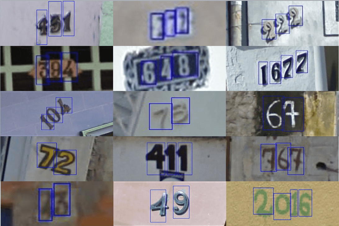
SVHN dataset (Street View House Numbers) is a real-world image dataset that is obtained by capturing house numbers from Google street view images.
The data used in this project is a subset of the original dataset (600,000 images of variable resolution). The subset is of 60,000 images (42,000 for training and 18,000 for validation). Each image is a single number at the center and most of these images have some digits cut at the sides. This can pose some distraction to the model training. The image data is a 32×32 RGB format much like MNIST data but more complex than it.
In this hands-on project, the python code is written from scratch. This is a multi-class classification with 10 classes from 0 to 9. We take an image from the dataset and find what the digit is. Digit 0 has label ‘0’, digit 1 has label ‘1’ and so on till digit 9, which has label ‘9’.
Python3 version has been used to execute code.
Learn how to statistically analyze and perform exploratory data analysis on a dataset before training a model.
Table of Content
- Import and mount Google Drive from google.colab library.
- Set Tensorflow version 2.x
- Import necessary libraries for algorithms and computations.
- Access data file stored in the drive with h5py library. Read and store the training and test variables. Close the file.
- Check the shape of the data sets (training and test).
- Display a random image from each of training and test sets to confirm if data is fetched correctly.
- Reshape the data columns from 32×32 to 1024 features/columns in the dataset as a single array of data is to be set for the model training for each instance. Check the target value percentage for classes 0 to 9.
- Perform a traditional machine learning classifier on the data set first.
- Apply KNN Classifier. Find an optimal value of n_neighbors and calculate the score on the validation set.
- As the data set is very huge, KNN algorithm takes too much time to find the optimal value of n_neighbors, so smaller training and validation subsets are created.
- Take in a value of n_neighbors that gives the best accuracy.
- Apply KNN algorithm on the original dataset using the optimal value of the hyperparameter and calculate its score on the original validation set.
- Compute confusion matrix on the 10 classes along with recall and precision.
- Note the observations.
- Define classes and functions for a deep neural network that will use activation layers and later batch normalization.
- Linear layer, ReLU activation layer, Batch normalization layer classes are created along with cross entropy and softmax. Stochastic gradient descent function performs the back propagation with gradient flow through all the layers in reverse order. The original batch is divided into multiple mini batches with shuffled images and then each minibatch data is made to pass through layers in feedforward method and then back propagated after the loss is computed.
- In backpropagation method, the gradients flow from the loss till the original input. Every trainable parameter is updated in the process.
- A deep neural network is created with linear layers followed by ReLU activation. The output layer outputs 10 classes.
- A test run is performed on this NN using a random learning rate and lambda.
- Batch normalization class is created with forward and backward functions.
- A second neural network is created with batch normalization layer added to it before every activation layer.
- The network is run using a learning rate of 1 and lambda of 0.0001.
- Test the network on a random image in the validation set.
- Compute and display confusion matrix along with recall and precision for the 10 classes.
- Note the observations.
#Import Drive from Google Colab
from google.colab import drive
drive.mount('/content/drive')
%tensorflow_version 2.x
Import the necessary libraries.
import pandas as pd
import numpy as np
from sklearn.metrics import accuracy_score, confusion_matrix, precision_score, recall_score, f1_score, precision_recall_curve, auc, precision_recall_fscore_support
import matplotlib.pyplot as plt
import h5py
from sklearn.neighbors import KNeighborsClassifier
Pandas library is used to create a dataframe to display recall and precision for the 10 classes. Numpy is used to create matrix, random numbers, dot product, etc. matplotlib is used to plot image from the pixel data.
Access data file in read mode.
h5f = h5py.File('/content/drive/My Drive/data.h5', 'r')
Read data into variables.
X_train = h5f['X_train'][:]
y_train = h5f['y_train'][:]
X_val = h5f['X_test'][:]
y_val = h5f['y_test'][:]
Now, that we have our training and validation variables set, close the file.
h5f.close()
print("Training set feature shape", X_train.shape)
print("Training set target shape", y_train.shape)
print("Validation set feature shape", X_val.shape)
print("Validation set target shape", y_val.shape)
The output comes as,
Training set feature shape (42000, 32, 32)
Training set target shape (42000,)
Validation set feature shape (18000, 32, 32)
Validation set target shape (18000,)
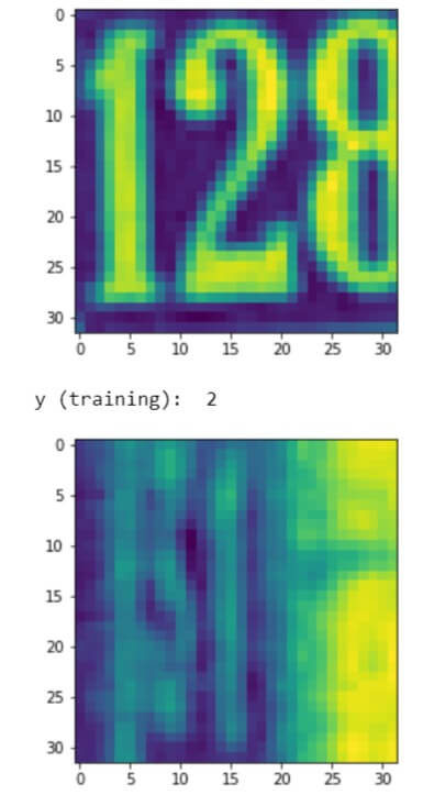
plt.imshow(X_train[0])Â Â #Show first image in the training set.
plt.show()
print('y (training): ', y_train[0])
plt.imshow(X_val[0])Â Â #Show first image in the validation set.
plt.show()
print('y (validation): ', y_val[0])
Reshape the features from 32×32 into a single dimensional array of 1024 features in total.
X_train = X_train.reshape(42000, 1024)
X_val = X_val.reshape(18000, 1024)
Normalize the data from 0-255 to 0-1 by dividing the inputs by 255. The denominator should be a float, else the output would become 0.
X_train = X_train / 255.0
X_val = X_val / 255.0
We should check the proportion of each class in the target variable to ensure there is no imbalance in the ground truth values.
for i in range(0,10):
    print("Label: {0} | Value % = {1}".format( i, (y_train[y_train == i].size / y_train.size)*100) )
It looks fine.
Check the shape of the variables before proceeding with training the k-Nearest model.
print(X_train.shape)
print(X_val.shape)
(42000, 1024)
(18000, 1024)
..and now all looks good to train the models.
knnX_train = X_train[0:10000, :]
knny_train = y_train[0:10000]
knnX_val = X_val[0:2000, :]
knny_val = y_val[0:2000]
print(knnX_train.shape)
print(knny_train.shape)
print(knnX_val.shape)
print(knny_val.shape)
As the dataset is very large, the computation involved in finding an optimal value of n-neighbours is taking too much time. To make it quick, subsets of smaller size are created and their shapes are as below.
(10000, 1024)
(10000,)
(2000, 1024)
(2000,)
knnScores = []
for i in range(20, 30):
    knn = KNeighborsClassifier(n_neighbors = i)
    #Fit the model
    knn.fit(knnX_train, knny_train)
    #Get the score
    knnScore = knn.score(knnX_val, knny_val)
    print("KNN Accuracy = {0} | n_neighbors = {1}".format(knnScore, i))
    #knnScore
    knnScores.append(knnScore)
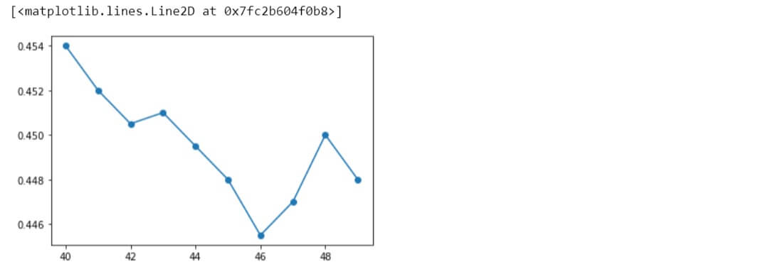
KNN Accuracy = 0.451 | n_neighbors = 20
KNN Accuracy = 0.4475 | n_neighbors = 21
KNN Accuracy = 0.447 | n_neighbors = 22
KNN Accuracy = 0.453 | n_neighbors = 23
KNN Accuracy = 0.451 | n_neighbors = 24
KNN Accuracy = 0.453 | n_neighbors = 25
KNN Accuracy = 0.4475 | n_neighbors = 26
KNN Accuracy = 0.4505 | n_neighbors = 27
KNN Accuracy = 0.455 | n_neighbors = 28
KNN Accuracy = 0.4505 | n_neighbors = 29
plt.plot(range(20,30), knnScores, 'o-')
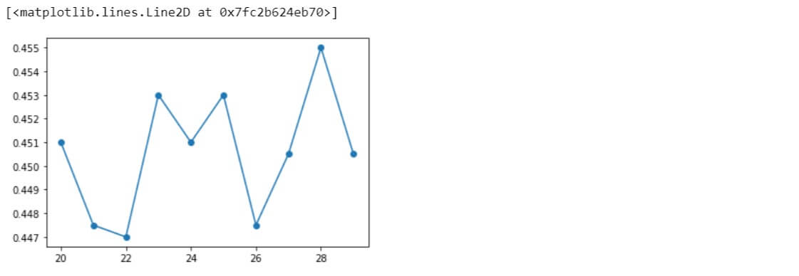
Similarly, other ranges of different values were also evaluated.
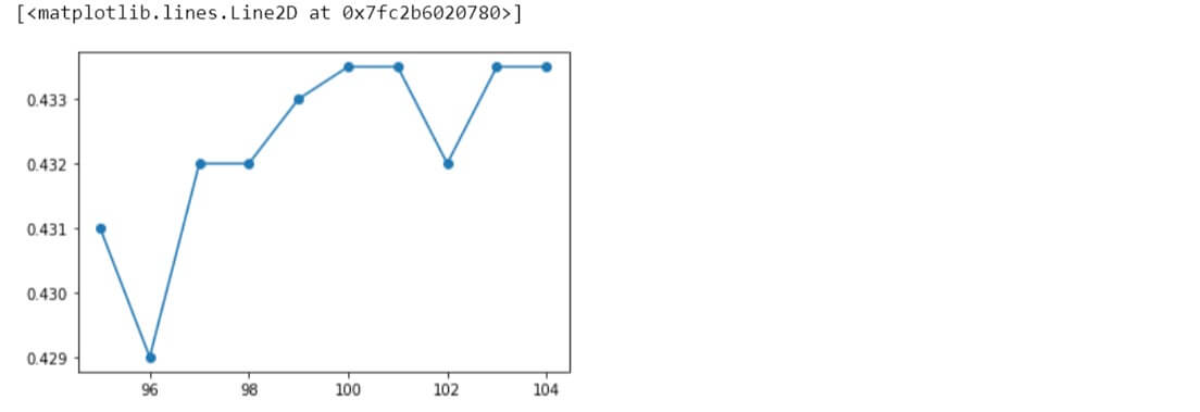
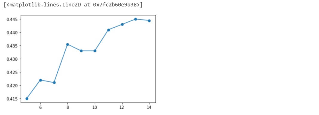
Taking the optimal value to be 28 for the hyperparameter, let us apply KNN algorithm to the original data variables with this value and see the performance.
So, the accuracy comes out to be 0.5319 on the validation set.
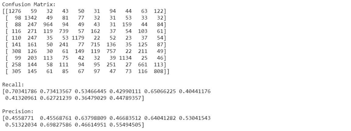
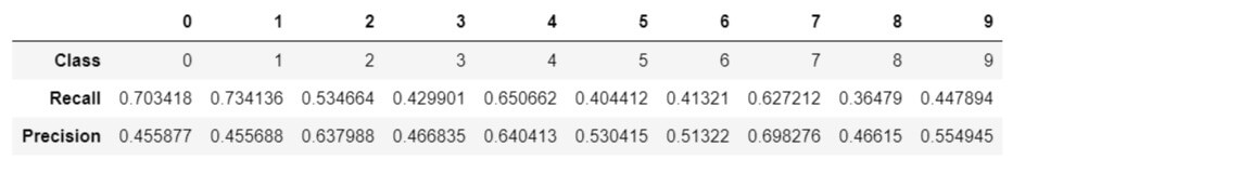
The class label ‘1’ has the best recall score of around 73% than the rest and the class label ‘7’ has the best precision score of around 69% than the rest.
The KNN classifier performed as expected, not good nor bad. In addition, it is also very computation heavy.
Now comes deep learning. Set up a neural network by adding layers to it. More the layers, the more non-linear the network will become and thus, better results.
class NN():
    def __init__(self, lossfunc=CrossEntropy(), mode='train'):
        self.params = []
        self.layers = []
        self.loss_func = lossfunc
        self.grads = []
        self.mode = mode

    def add_layer(self, layer):
        self.layers.append(layer)
        self.params.append(layer.params)

    def forward(self, X):
        for layer in self.layers:
            X = layer.forward(X)
        return X

    def backward(self, nextgrad):
        self.clear_grad_param()
        for layer in reversed(self.layers):
            nextgrad, grad = layer.backward(nextgrad)
            self.grads.append(grad)
        return self.grads

    def train_step(self, X, y):
        out = self.forward(X)
        loss = self.loss_func.forward(out,y)  + ((Lambda / (2 * y.shape[0])) * np.sum([np.sum(w**2) for w in self.params[0][0]]))
        nextgrad = self.loss_func.backward(out,y) + ((Lambda/y.shape[0]) * np.sum([np.sum(w) for w in self.params[0][0]]))
        grads = self.backward(nextgrad)
        return loss, grads

    def predict(self, X):
        X = self.forward(X)
        p = softmax(X)
        return np.argmax(p, axis=1)

    def predict_scores(self, X):
        X = self.forward(X)
        p = softmax(X)
        return p

    def clear_grad_param(self):
        self.grads = []
ReLU activation function is to be used between other linear layers. Cross entropy and softmax functions are to be used to calculate loss within the epochs. Define each layer with forward and backward functions and add them to the neural network.
Stochastic gradient descent method is used to traverse forward and backpropagate across layers with the gradients to update in the process and find the minimum loss at the output. The step size is defined by a learning rate value.
def sgd(net, X_train, y_train, minibatch_size, epoch, learning_rate, mu=0.5, X_val=None, y_val=None, Lambda=0, verb=True):
    val_loss_epoch = []
    train_loss_epoch = []
    minibatches = minibatch(X_train, y_train, minibatch_size)
    minibatches_val = minibatch(X_val, y_val, minibatch_size)
    for i in range(epoch):
        if( len(train_loss_epoch) > 2 ):
            if( (train_loss_epoch[len(train_loss_epoch)-1]) - (train_loss_epoch[len(train_loss_epoch)-2]) > 0 ):
                if learning_rate >= 0.0001 :
                    learning_rate = learning_rate/10;

        loss_batch = []
        val_loss_batch = []
        velocity = []
        for param_layer in net.params:
            p = [np.zeros_like(param) for param in list(param_layer)]
            velocity.append(p)

        # iterate over mini batches
        for X_mini, y_mini in minibatches:
            loss, grads = net.train_step(X_mini, y_mini)
            loss_batch.append(loss)
            update(velocity, net.params, grads, learning_rate=learning_rate, mu=mu)

        for X_mini_val, y_mini_val in minibatches_val:
            val_loss, _ = net.train_step(X_mini, y_mini)
            val_loss_batch.append(val_loss)

        # accuracy of model at end of epoch after all mini batch updates
        m_train = X_train.shape[0]
        m_val = X_val.shape[0]
        y_train_pred = []
        y_val_pred = []
        y_train1 = []
        y_vall = []
        for ii in range(0, m_train, minibatch_size):
            X_tr = X_train[ii:ii + minibatch_size, : ]
            y_tr = y_train[ii:ii + minibatch_size,]
            y_train1 = np.append(y_train1, y_tr)
            y_train_pred = np.append(y_train_pred, net.predict(X_tr))

        for ii in range(0, m_val, minibatch_size):
            X_va = X_val[ii:ii + minibatch_size, : ]
            y_va = y_val[ii:ii + minibatch_size,]
            y_vall = np.append(y_vall, y_va)
            y_val_pred = np.append(y_val_pred, net.predict(X_va))

        train_acc = check_accuracy(y_train1, y_train_pred)
        val_acc = check_accuracy(y_vall, y_val_pred)

        ## weights
        w = np.array(net.params[0][0])

        ## adding regularization to cost
        mean_train_loss = (sum(loss_batch) / float(len(loss_batch)))
        mean_val_loss = sum(val_loss_batch) / float(len(val_loss_batch))

        train_loss_epoch.append(mean_train_loss)
        val_loss_epoch.append(mean_val_loss)

        if verb:
            #if i%50==0:
            print("Epoch {3}/{4}: Loss = {0} | LR = {5} | Mu = {6} | Training Accuracy = {1} | Validation Accuracy = {2}".format(mean_train_loss, train_acc, val_acc, i+1, epoch, learning_rate, mu))
    return net, val_acc
def NN1(iterations, lr, lambdaa = 0, verb=True):
    input_dim = X_train.shape[1]
    ## hyperparameters
    iterations = iterations
    learning_rate = lr
    hidden_nodes = 10
    output_nodes = 10
    ## define neural net
    nn = NN()
    nn.add_layer(Linear(input_dim, 50))
    nn.add_layer(ReLU())
    nn.add_layer(Linear(50, 20))
    nn.add_layer(ReLU())
    nn.add_layer(Linear(20, output_nodes))
    nn, val_acc = sgd(nn, X_train , y_train, minibatch_size=1000, epoch=iterations, learning_rate=learning_rate, X_val=X_val, y_val=y_val, Lambda=Lambda, verb=verb)
    return nn, val_acc
net, val_acc = NN1(200, lr = 2)
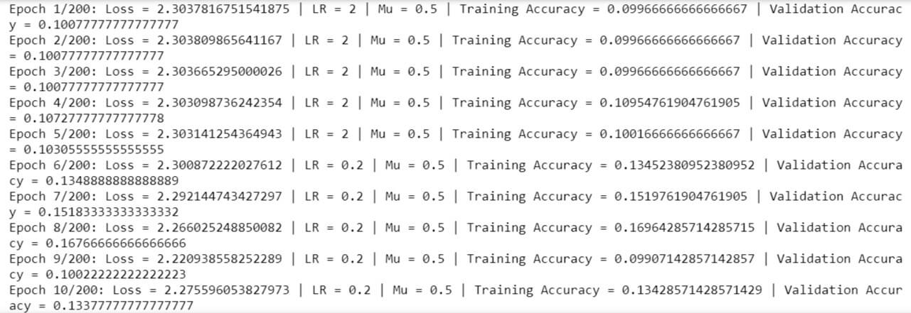
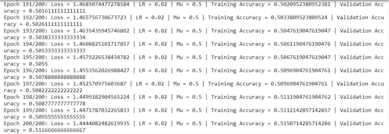
The loss decreases gradually and gets to a value of ~0.51 after 200 epochs.
Implement Batch Normalization
class BatchNormalization():
    #Initialize class variables
    def __init__(self, size):
        self.gamma = np.ones(size).T #shape = (size,)
        self.beta = np.ones(size).T * 0.1 #shape = (size,)
        self.eps = 1e-6
        self.params = [self.gamma, self.beta]
        self.dX = None
        self.dgamma = None
        self.dbeta = None

    def forward(self, X):
        N, D = X.shape
        #Calculate mean
        mean = 1./N * np.sum(X, axis = 0)
        #Subtract mean vector of every trainings example
        self.X1 = X - mean
        #Following the lower branch - calculation denominator
        sq = self.X1 ** 2
        #Calculate variance
        self.var = 1./N * np.sum(sq, axis = 0)
        #Add eps for numerical stability, then sqrt
        self.sqrtvar = np.sqrt(self.var + self.eps)
        #Invert sqrtwar
        self.ivar = 1./self.sqrtvar
        #Execute normalization
        self.Xhat = self.X1 * self.ivar
        #Nor the two transformation steps
        gammaX = self.gamma * self.Xhat
        #Calculate and return output
        out = gammaX + self.beta
        return out

    def backward(self, nextgrad):
        #Get the dimensions of the input/output
        N,D = nextgrad.shape
        self.dbeta = np.sum(nextgrad, axis=0)
        dgammax = nextgrad #not necessary, but more understandable
        self.dgamma = np.sum(dgammax*self.Xhat, axis=0)
        dxhat = dgammax * self.gamma
        divar = np.sum(dxhat*self.X1, axis=0)
        dxmu1 = dxhat * self.ivar
        dsqrtvar = -1. /(self.sqrtvar**2) * divar
        dvar = 0.5 * 1. /np.sqrt(self.var+self.eps) * dsqrtvar
        dsq = 1. /N * np.ones((N,D)) * dvar
        dxmu2 = 2 * self.X1 * dsq
        dx1 = (dxmu1 + dxmu2)
        dmu = -1 * np.sum(dxmu1+dxmu2, axis=0)
        dx2 = 1. /N * np.ones((N,D)) * dmu
        self.dX = dx1 + dx2
        return self.dX, [self.dgamma, self.dbeta]
def NN2(iterations, lr, lambdaa = 0, verb=True):
    input_dim = X_train.shape[1]
    Lambda = 0
    Lambda = lambdaa
    ## hyperparameters
    iterations = iterations
    learning_rate = lr
    hidden_nodes = 10
    output_nodes = 10
    ## define neural net
    nn = NN()
    nn.add_layer(Linear(input_dim, 50))
    nn.add_layer(BatchNormalization(50))
    nn.add_layer(ReLU())
    nn.add_layer(Linear(50, 20))
    nn.add_layer(BatchNormalization(20))
    nn.add_layer(ReLU())
    nn.add_layer(Linear(20, output_nodes))
    nn, val_acc = sgd(nn, X_train , y_train, minibatch_size=1000, epoch=iterations, learning_rate=learning_rate, X_val=X_val, y_val=y_val, Lambda=Lambda, verb=verb)
    return nn, val_acc
net, val_acc = NN2(1000, lr = 1, lambdaa = 0.0001)
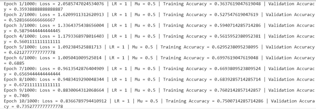
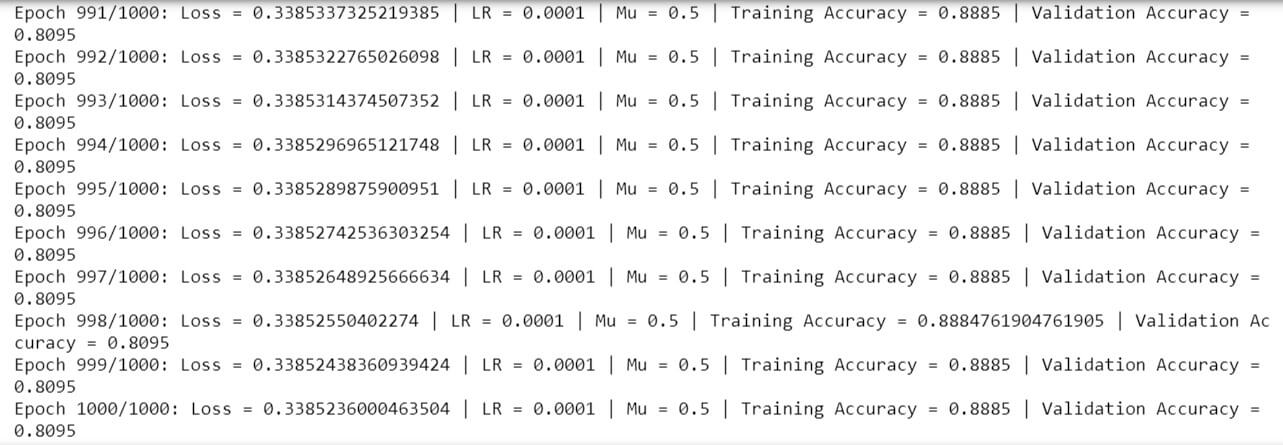
An accuracy of ~81% is achieved on the validation set after running a thousand epochs.
Test a random image from the validation set and see what the network predicts.
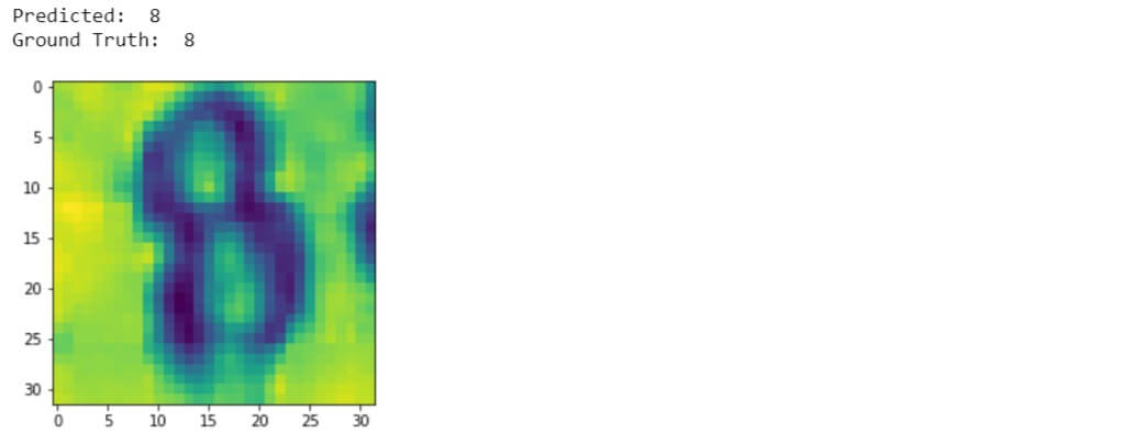
Compute the classification metric report.
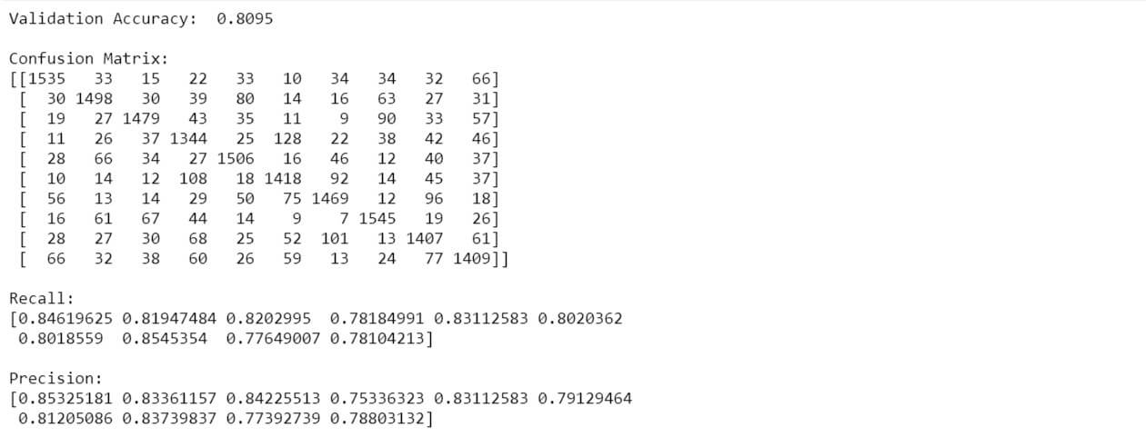
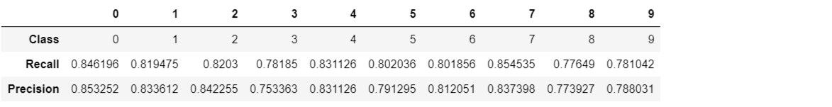
Looking at class level accuracy, both recall and precision came out good, in the range of 75% to 85%. Recall is least for class labelled ‘8’ and maximum for class labelled ‘7’. Precision is least for class labelled ‘3’ and maximum for class labelled ‘0’.
Compared to the neural network without batch normalization, this neural network is much quicker and achieved higher accuracy in less time. Compared to the KNN classifier, this neural network is much more accurate and much more quicker.
With traditional machine learning algorithms on image detection, it seems like they perform up to a level of accuracy and could not go beyond that as we saw using the KNN classifier, for which an optimal value of n_neighbors was determined, and 53% accuracy is what it came out with.
Batch normalization is the key that makes the difference between the 2 neural networks used. It helps in normalizing the input and provide unit gaussians in the output, thereby reducing the loss very quickly.
A deeper neural network layer performs better than a shallow network as it makes the network more non linear.
With a high learning rate, we cannot expect much loss after a certain point, whereas with a smaller learning rate, we can expect to achieve a much smaller loss but with a higher number of epochs and slow speed.
The approach to divide the learning rate by 10 whenever the loss increases works. With this approach, the network was able to find the minimum loss in a shorter time and lesser epochs.
The project acknowledges http://ufldl.stanford.edu/housenumbers/ for the dataset and reference.